Applied Computational Economics and Finance
Solutions to Exercises using Stata and Mata
The excellent book Applied Computational Economics and Finance by Mario J. Miranda and Paul L. Fackler (MIT Press, 2002) provides numerous well-designed exercises for those studying the book to solidify their understanding and work with applications. Unfortunately, the book does not come with a solutions manual, nor have we found one online (if you have, please tell us!). Much of the discussion in the book refers programs the authors wrote for the book in Matlab. And the book's CompEcon toolkit provides these Matlab programs.We prefer to use Stata and its integrated matrix programming language Mata. We set for ourselves here an exciting challenge--to work through the exercises in the book, adapt the solutions and code to Stata and Mata, and share the results with our readers. Let's see how far we get.
We will be storing code for this project at our CompEcon GitHub repository.
Solutions to Chapter 1 exercises
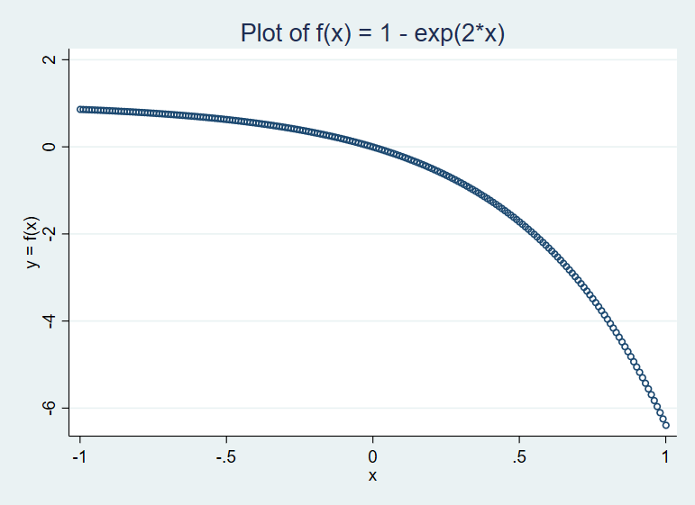
We will avoid copying the exercise question itself in our solution, and instead encourage readers to refer to their personal copy or to buy the book.Exercise 1.1. Plot a function on a fixed interval
*Create a variable x from -1 to 1 in steps of 0.01 (201 values for x)
range x -1 1 201
gen y = 1 - exp(2*x)
label var y "y = f(x)"
*Make scatter plot
scatter y x, title("Plot of f(x) = 1 - exp(2*x)") msymbol(oh)
Exercise 1.2. Produce a matrix product (standard matrix product and element-by-element multiplication) and solve a linear equation
. matrix A = ( 0, -1, 2 \ -2, -1, 4 \ 2, 7, -3)

. matrix B = (-7, 1, 1 \ 7, -3, -2 \ 3, 5, 0)

. matrix y = (3 \ -1 \ 2)

. mat list A

A[3,3]
    c1  c2  c3
r1   0  -1   2
r2  -2  -1   4
r3   2   7  -3

. mat list B

B[3,3]
    c1  c2  c3
r1  -7   1   1
r2   7  -3  -2
r3   3   5   0

. mat list y

y[3,1]
    c1
r1   3
r2  -1
r3   2

.
. *a. Produce matrix C = A*B using standard matrix product
. matrix C = A*B

. mat list C

C[3,3]
     c1   c2   c3
r1   -1   13    2
r2   19   21    0
r3   26  -34  -12

. *Solve Cx = y for x.
. matrix x = inv(C)*y

. mat list x

x[3,1]
            c1
c1  -1.1153846
c2   .96153846
c3  -5.3076923

.
. *b. Produce matrix C = A*B using element-by-element matrix product
. *In stata this is done using the Halamard product function
. matrix C = hadamard(A, B)

. mat list C

C[3,3]
     c1   c2   c3
r1    0   -1    2
r2  -14    3   -8
r3    6   35    0

. *Solve Cx = y for x.
. matrix x = inv(C)*y

. mat list x

x[3,1]
            c1
c1  -.79958678
c2   .19421488
c3   1.5971074
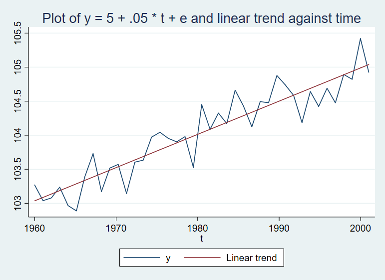
Exercise 1.3. Using a standard normal pseudo-random number generator, simulate and plot a time-series
. clear

. *Generate a variable t for time ranging from 1960 to 2001
. range t 1960 2001 41
number of observations (_N) was 0, now 41

. *Generate a random error term with mean 0 and SD 0.2
. gen e = rnormal(0, 0.2)

. *Create time series y as a function of time and the error term
. gen y = 5 + .05 * t + e

. summarize

    Variable |        Obs        Mean    Std. Dev.       Min        Max
-------------+---------------------------------------------------------
           t |         41      1980.5    12.27863       1960       2001
           e |         41    .0122709    .2427657  -.4537043   .4329219
           y |         41    104.0373    .6465939    102.889   105.4206

. *Generate a linear trend line by regressing y on a constant and time and plot
. *The easy way to do this is fit the trend using regress y t, then get predicted y.
. *But here, the book wants us to use the "manual" approach with matrices to build the skills for more complex calculations.

. *So first we make a matrix y containing our variable y
. mkmat y, matrix(y)
. *Then make a matrix t
. mkmat t, matrix(t)
. *Make a column vector of ones
. matrix ones = J(41, 1, 1)
. *Join the columns of the constant term and time into matrix X
. matrix X = ones , t
. *Create the coefficient vector using linear regression
. matrix b = inv(X' * X) * X' * y
. *Create the trend line as the regression prediction
. matrix yhat = X * b
. *Save vector yhat as a variable in Stata
. svmat yhat
. label var yhat "Linear trend"
. line y yhat t, title("Plot of y = 5 + .05 * t + e and linear trend against time")
Exercise 1.4. Solve for the equilibrium of a rational expectations commodity market with a simple two-point distribution for the key random variable
For an agricultural product, the acerage planted (a) depends on the expected price (Ep) at harvest:a = 0.5 + 0.5*Ep
Yield (y) is uncertain, but given its realization, the quantity (q) produce is:
q = a * y
The demand curve for the product is:
p = 3 - 2q
The rational expectations equilibrium is the pair p*, q* that clears the market (quantity supplied = quantity demand) and is consistent with expectations given the uncertainty over yield. Suppose y can take two values, 0.7 and 1.3, each with probability 0.5.
a. Without goverment support payments, substituting (1) into (2) and (2) into (3) we get:
p = 3 - 2(0.5 + 0.5*Ep) * y
Taking expectations of both sides, given E(y) = 0.5*0.7 + 0.5*1.3 = 1, gives
Ep = 3 - 2(0.5 + 0.5*Ep)
Ep = 3 - 1 - Ep
Ep = 1
With rational expectations, acerage will be set according to the expected price, so a=1. The realized price will vary, depending on realized yield and quantity. The variance of price, Var(p) = E(p^2) - (Ep)^2, can be computed by considering the two cases.
If yield = 0.7, then p = 3 - 2(0.7) = 1.6
If yield = 1.3, then p = 3 - 2(1.3) = 0.4
Then Var(p) = 0.5 * 0.4^2 + 0.5 * 1.6^2 - 1
Var(p) = 0.36
b. With government support payments, even using the simple two point distribution for yield, the basic problem is taking the expectation over the max operator when its argument, p, is endogenous to the system. So rather than attempt an analytic solution, we will we adapt the MATLAB program on page 4 to Stata.
*Possible values for yield in vector y
matrix y = [0.7, 1.3]
*Probability over those values in vector w
matrix w = [0.5, 0.5]
matrix ones = [1 , 1]
*Start with initail value of a=1
scalar a = 1
*Try 10 iterations and see if that is enough
forvalues i = 1(1)10 {
	*Compute prices, given a and demand curve, under each realization of y
	matrix p = 3*ones - 2*a*y
	*Regular Stata does not have a max function over a matrix, we do next step directly
	*Computing the expected producer price given a
	scalar f = w[1,1]*max(p[1,1], 1) + w[1,2]*max(p[1,2], 1)
	*Compute expected market price
	matrix wp=w'*p
	*Compute updated a given expected producer price
	scalar a = 0.5 + 0.5 * f
	disp "a = " a, "wp = " wp[1,1], "f = " f
}
mat list p
*Variance of producer price is
disp 0.5*(max(p[1,1], 1))^2 + 0.5*(max(p[2,1], 1)) - f^2
Output of program:
a = 1.15 wp = .8 f = 1.3
a = 1.0975 wp = .695 f = 1.195
a = 1.115875 wp = .73175 f = 1.23175
a = 1.1094438 wp = .7188875 f = 1.2188875
a = 1.1116947 wp = .72338938 f = 1.2233894
a = 1.1109069 wp = .72181372 f = 1.2218137
a = 1.1111826 wp = .7223652 f = 1.2223652
a = 1.1110861 wp = .72217218 f = 1.2221722
a = 1.1111199 wp = .72223974 f = 1.2222397
a = 1.111108 wp = .72221609 f = 1.2222161
. mat list p
p[1,2]
           c1         c2
r1  1.4444322  .11108834

. *Variance of producer price is
. disp 0.5*(max(p[1,1], 1))^2 + 0.5*(max(p[2,1], 1)) - f^2
.04937999
Comparing the equilibrium outcomes with and without the government price support, we observe higher acerage planted, a higher expected price to producers, and a lower expected price to consumers. Also, the variance of the producer price is lower with the price support policy.
c. The government subsidy per unit is the difference between the producer price and market price. Multiply that by the quantity to get the subsidy. Then divide by equilbrium acres planted. Take expected value over each case for yield. With probability 0.5, the subsidy is 0. So we have:
. disp (0.5 * (max(p[1,1], 1) - p[1,1]) * a * y[1,1] + 0.5 * (max(p[1,2], 1) - p[1,2]) * a * y[1,2])/a
.57779258